In ion mobility spectrometry (IMS), the resolving power of mobility measurements scales with the square root of the drift tube length at a constant electric field. This complicates the miniaturization of IMS devices. An IMS instrument with circular geometry has been developed to address this issue, by increasing the resolving power without dramatically increasing the size of the instrument. The circular drift tube operates by transporting a packet of ions of a defined mobility around the circle a number of cycles. To date, a packet of ions has been cycled 100 ¾ times, corresponding to a drift length of 183 meters.
Note: 183 m is approximately 200 yards, twice the total distance from endzone to endzone on a standard American football field. Although no official records for the 200 yard dash are available, the record for running the 200 meter (~220 yards) sprint is ~19.2 seconds for Olympic sprinters, and ~21 seconds for collegiate football players. Typical drift times (for substance P) at 100 ¾ cycles are ~1.2 seconds, resulting in a theoretical time for the 200 m sprint of ~1.3 seconds.
The ion cyclotron mobility spectrometry instrument operates in the following manner, based on scanning the frequency used to apply a drift field to segmented regions of a circular drift tube. Ions with mobilities that are resonant with the field application frequency are transmitted while non-resonant species are eliminated. This allows only ions of given mobilities to be analyzed, while others are eliminated. If a small packet of ions is introduced into the drift tube only one segment of the drift tube is filled; or multiple packets are introduced allowing the filling of multiple segments. The stepwise filling of these segments can be accomplished by incrementally increasing the width of the ion packet pulsed into the drift tube or by pulsing in multiple smaller packets at the same field application frequency of the drift tube. Each segment is sequentially filled according to the drift field application frequency and the width of the injection pulse. Mobility separation is demonstrated with a drift field frequency spectrum obtained by scanning the drift field application frequency and recording the ion current. The isolation of ions according to their mobilities and their confinement in the circular drift tube for extended periods of time is analogous to an ion trap device.
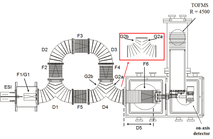
An instrument diagram is shown with ions generated by electrospray ionization (ESI) collected in a hourglass ion funnel (F1). Periodically packets of ions are pulsed into the circular drift tube containing eight distinct regions each operated at 8 V⋅cm–1. These include four curved drift regions (labeled D1–D4) and four ion funnels (labeled F2–F5). After D4 there is a short drift region operated at 9 V⋅cm–1; followed by F6 operated at 11 V⋅cm–1. Upon exiting F6, ions are then focused through a series of ion optics before being mass analyzed and detected.
There are two lenses in D4 (labeled G2a and G2b) that are isolated from the rest of the drift assembly and obtain their voltages from an external pulse generator. Ions can be transmitted around numerous cycles by switching the voltages of G2a and G2b at the appropriate time.
A home-built drift field wavedriver controls the drift field for each of the individual drift regions (D1–D4) and ion funnels (F2–F5). The field across the drift region remains constant by varying the bias of the D and F regions. Ions are propagated around the drift tube by periodically applying two separate fields to distinct sections of the drift tube. A packet of ions is introduced into the D1 region during one field application setting, and, after a specified delay, the field application setting is switched and ions can travel into the F2 region. Upon switching fields again, ions can travel into the D2 region. Ions traveling beyond or those not reaching D2 before the next field application setting are eliminated.
With each field transition, ions at the leading and trailing edges of the transmission packet are eliminated, leaving only a narrow range of mobilities. The period of the wavedriver corresponds to the time required for ions to travel the length of one curved region and one ion funnel, which allows for the reduced mobility of the peak to be determined from the following relation, where lt and le are the lengths of the ion transmission and ion elimination regions, respectively. E is the electric field, f is the drift field application frequency (inverse of the wavedriver period), and T and P are the temperature and pressure, respectively, of the drift buffer gas.

![]() Copyright © 2012 The Trustees of Indiana University | Copyright Complaints
Copyright © 2012 The Trustees of Indiana University | Copyright Complaints