The Group has previously developed a simple split-field drift tube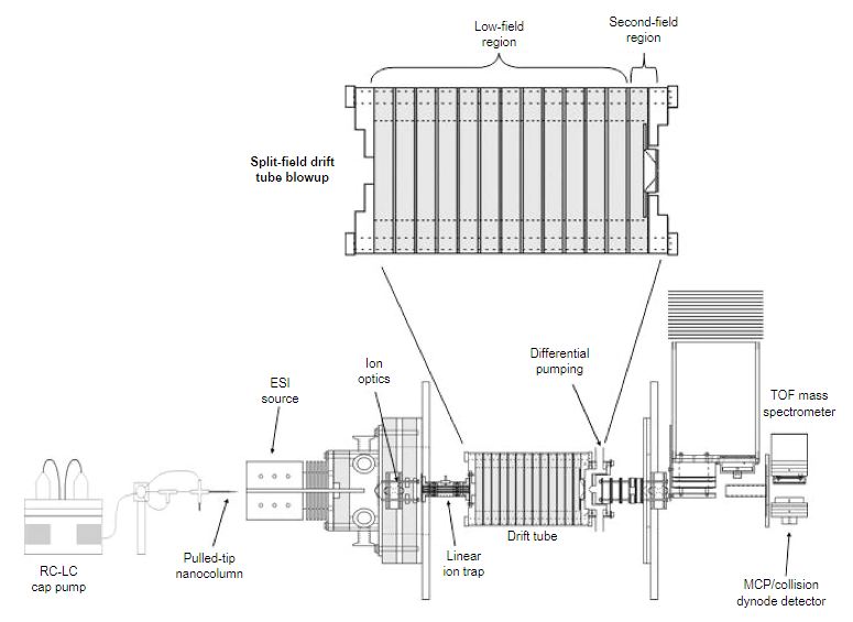
A simple split-field drift tube design. See Pub. 99 for more information. for ion mobility/mass spectrometry. This early instrumental design allowed for mixtures of precursor ions to be separated in a low-field region before being exposed to a short variable-field region prior to mass analysis. When this variable-field region was operated at an applied field equivalent to that of the drift region, the precursor ions would be allowed into the mass analyzer. When the applied fields in this variable-field region were increased, the precursor ions could be fragmented prior to mass analysis, and then by modulating these low- and high-field conditions, mass spectra for both precursor and fragment ions could be obtained for complex mixtures of ions without initial mass selection.
Further development of this idea led to the constuction of a new IMS instrument that allows a mixture of precursor ions to be dispersed based upon differences in mobility. Once dispersed, it is then possible to select an ion of a specific mobility and subject it to further collisional activation resulting in fragmentation of the precursor ion, changes in the conformation of the ions, or in certain instances, both. These new fragment ions (or conformers) are then allowed to separate again in a second (or third) low-field region prior to mass analysis. This IMS–IMS approach is analogous in many ways to MS–MS strategies; however, the separations of the initial precursor and first dissociation products are based on cross section-to-charge (Ω/z) rather than mass-to-charge (m/z) ratios.
Note: Both of our current linear IMS instruments are capable of multidimensional IMS experiments, however, for the purposes of this discussion, the experimental summary focuses on the use of our longer 3m instrument as opposed to the original 2m apparatus. More information about the 2m instrument can be found here.
Briefly, a continuous beam of electrosprayed ions is introduced directly into an ion funnel region (F1) and accumulated. Periodically the concentrated ion packet is gated into the first drift tube (D1). The drift tube contains 3 Torr He buffer gas; ions migrate across the tube under the influence of a weak electric field, and different species separate due to differences in their mobilities through the gas. As ions exit the first drift region, they enter another ion funnel that is used to radially focus the diffuse ion clouds and transmit species into the front of a second drift region (D2). The entrance of D2 contains an ion gate and ion activation region such that it is possible to select and energize specific components of the ion mixture. There is a third drift region (D3) that operates in an analogous fashion. Ions exit the drift tube into a vacuum chamber and are focused into a time-of-flight mass spectrometer for m/z analysis.
The entire drift tube assembly is ~300 cm long. Ions are selectively gated by raising or lowering fields in the gate regions (G1–G3), as shown in Figure 1 at specific delay times that are controlled by a pulse delay generator. Collisional activation in any activation region (IA1, IA2, or IA3) is achieved by increasing the voltage between the last two lenses of each funnel.
Another way to visualize multi-dimensional IMS instrumentation is shown below using a theoretical protein ion. If the animation progresses too fast, an alternate collection of images can be found here.

It is instructive to highlight several example datasets from our previous multidimensional IMS experiments. These types of experiments are extremely varied, allowing for a wealth of potential information to be obtained.
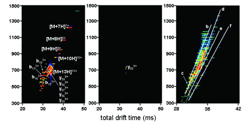
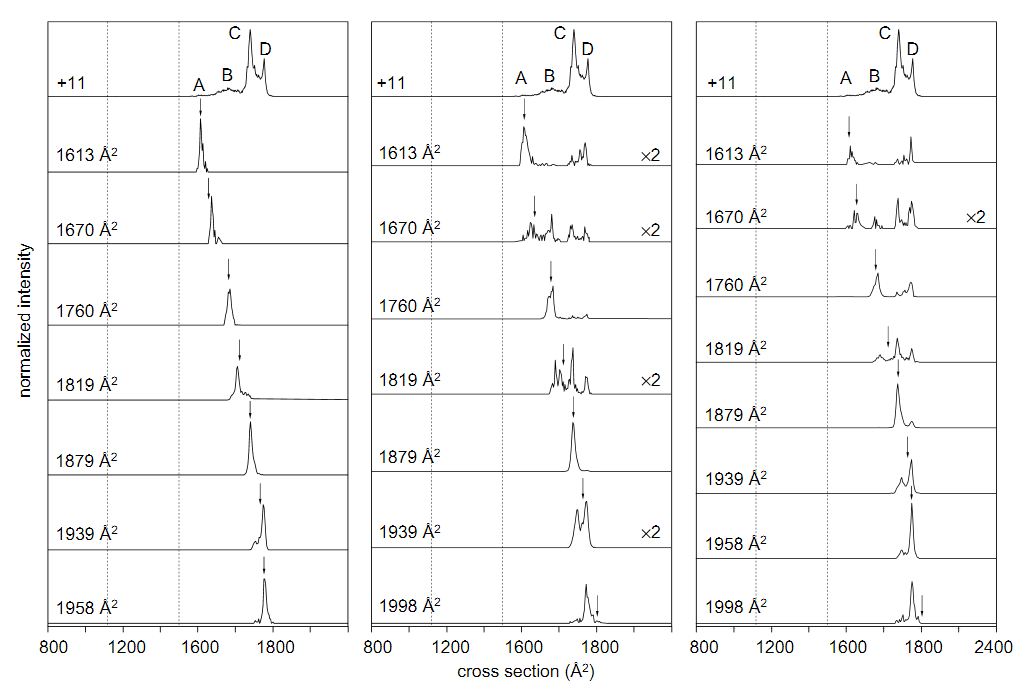
More information and discussion of these figures can be found in the associated references listed below, all of which can also be found on the Publications page as well.