Clemmer Group

Research | Instrumentation

1. Nested IMS–TOFMS
   • Figure 1
   • Figure 2
2. Multidimensional IMS
3. Circular Drift Tube
   • Figure 3
   • Equation 1
4. IMS–hν–Q Instrument
   • Figure 4
5. References

Nested IMS–TOFMS

Jason Grosch

Nested ion mobility mass spectrometry (IMS–MS) measurements are the simultaneous detection of the IMS drift time and mass spectrum of the analyte ions. Ion mobility measurements are typically on the millisecond (ms) timescale and flight times occur on the order of microseconds (μs), which allows for a complete mass spectrum to be taken for each drift bin. The two-dimensional plot of m/z against drift time is referred to as the nested IMS–MS distribution.

The IMS–MS technique has great advantage in differentiating ions of the same m/z. Prior to the advent of nested IMS–MS, the standard method of collecting mass spectra and ion mobility distributions was to transmit a narrow m/z window.1, 2 For complex mixtures with multiply charged ion distributions, such as those from electrospray ionization (ESI), separate ion mobility distributions must be recorded for each m/z ion.1 These types of measurements are low through-put measurements because ions that are not selected are discarded. In 1998 the we developed the nested IMS–MS technique, resulting in the capability to measure both mass spectra and drift distributions of any m/z ions continuously and simultaneously.3 The nested IMS–MS design established a new paradigm in the IMS field by eliminating the need to measure individual ion distributions for each m/z ion.

Ions that travel through an IMS mobility cell experience collisions with a neutral buffer gas (typically He or N2) and separate based upon differences in mobility, a constant determined by ion-neutral interactions. Some of the physical properties of ions that influence mobility are charge, shape (or, conformation), polarizability, and (to a limited extent) mass. As such, IMS–MS is especially applicable to study fundamental structural properties of gas-phase ions such as proteins, lipids, carbohydrates, and polymers.

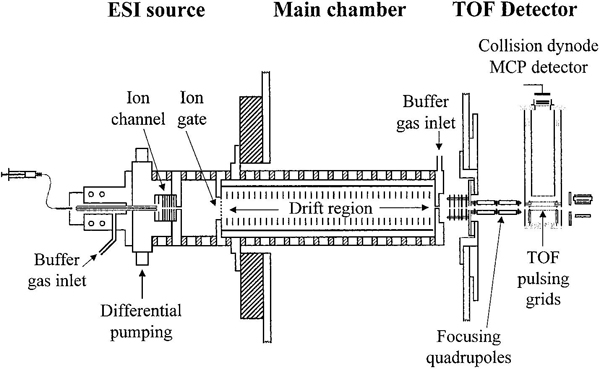
An early design of an IMS–MS instrument utilizing an orthogonal TOF is shown below.4 More information about the early development of these instruments, including archived photographs and schematics, can be found here.

Figure 1: Schematic diagram of the high-resolution ion mobility time-of flight mass spectrometer. For more information, refer to Publication #52.

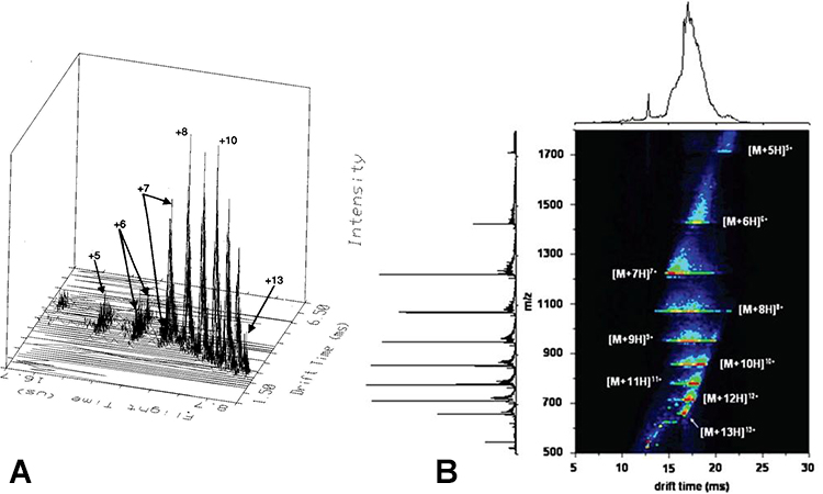
Examples of nested IMS–MS distributions are shown below in Figure 2. To the left (A)5 is one of the original nested plots, showing ion intensity as a function of drift time and time of flight, and to the right (B)6 is a modern nested IMS–MS distribution showing intensity (contoured) as a function of drift time and m/z.

Figure 2: (A) Three-dimensional representation of drift time, flight time, and ion abundances for a distribution of electrosprayed ubiquitin ions. The drift tube was operated using a drift field of 14.53 V·cm-1, under 2.059±0.006 Torr of He buffer gas. This spectrum was recorded using an injection voltage of 80 V. For more information, refer to Publication #46. (B) Nested drift(flight) time distributions showing the total distribution of electrosprayed ubiquitin ions. Also shown are the summed mass spectra (side) and summed drift time distributions(top) obtained by integrating the two-dimensional data across all drift times and all m/z values, respectively. The drift time represents the total time required for the ions to travel through D1 to the TOF source. For more information, refer to Publication #110.

Multidimensional IMS

Nicholas A. Pierson

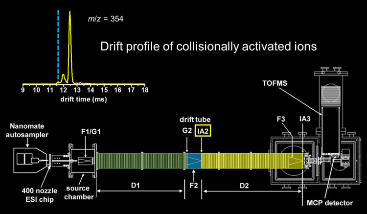
Our laboratory developed multidimensional IMS in 2006.7 We have applied this technology in two general areas 1) probing ion structure8, 9, 10, 11, 12, 13, 14, 15 and 2) complex mixture analysis.16, 17, 18, 19, 20, 21, 22, 23 The idea is this: regardless of high-resolution mobility separation, chemical interferences still exist for mobility-matched ions. In multidimensional IMS, the drift tube is divided up into discrete drift regions separated by ion selection and ion activation regions.

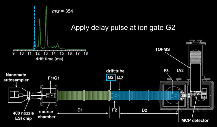
Following conventional IMS separation through a given drift region, a narrow packet of mobility-matched ions is isolated by momentarily lowering a repulsive potential at the electrostatic gate at a given delay time.

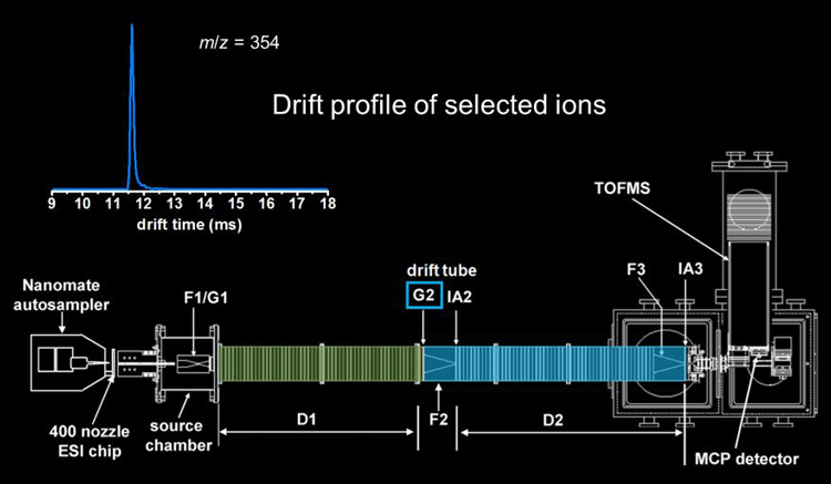
The selected ions are then subjected to collisional activation (ion�neutral collisions with the He buffer gas) by increasing the electric field in the ion activation region. This ion activation step can cause some of the ions to anneal to more compact structures, some of the ions to anneal to more elongated structures, and some of the ions remain the same. In addition to changing structure, higher activation voltages can be used to dissociate selected ions by CID.

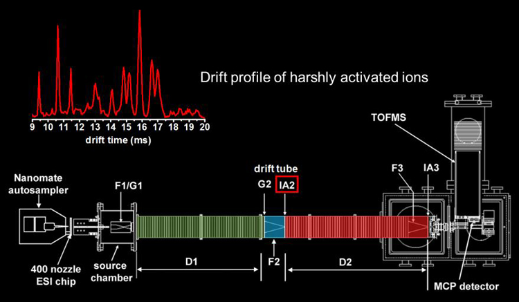
No longer uniformly mobility matched, the ions are then separated in the following drift region. We have demonstrated both two- and three-dimensional IMS. Higher-throughput multidimensional IMS can be achieved through a technique called combing.6 Pictures of the linear instruments typically used for these experiments can be found here for the 2m version and here for the longer 3m version.

Circular Drift Tube

Rebecca Glaskin

In IMS, the resolving power of mobility measurements scales with the square root of the drift tube length at a constant electric field. This complicates the miniaturization of IMS devices. An IMS instrument with circular geometry has been developed23, 24 to address this issue, by increasing the resolving power without dramatically increasing the size of the instrument. The circular drift tube operates by transporting a packet of ions of a defined mobility around the circle a number of cycles. To date, a packet of ions has been cycled 100 ¾ times, corresponding to a drift length of 183 meters.

Note: 183 m is approximately 200 yards, twice the total distance from endzone to endzone on a standard American football field. Although no official records for the 200 yard dash are available, the record for running the 200 meter (~220 yards) sprint is ~19.2 seconds for Olympic sprinters, and ~21 seconds for collegiate football players. Typical drift times (for substance P) at 100 ¾ cycles are ~1.2 seconds, resulting in a theoretical time for the 200 m sprint of ~1.3 seconds.

The ion cyclotron mobility spectrometry instrument operates in the following manner, based on scanning the frequency used to apply a drift field to segmented regions of a circular drift tube. Ions with mobilities that are resonant with the field application frequency are transmitted while non-resonant species are eliminated. This allows only ions of given mobilities to be analyzed, while others are eliminated. If a small packet of ions is introduced into the drift tube only one segment of the drift tube is filled; or multiple packets are introduced allowing the filling of multiple segments. The stepwise filling of these segments can be accomplished by incrementally increasing the width of the ion packet pulsed into the drift tube or by pulsing in multiple smaller packets at the same field application frequency of the drift tube. Each segment is sequentially filled according to the drift field application frequency and the width of the injection pulse. Mobility separation is demonstrated with a drift field frequency spectrum obtained by scanning the drift field application frequency and recording the ion current. The isolation of ions according to their mobilities and their confinement in the circular drift tube for extended periods of time is analogous to an ion trap device.

Figure 3: Schematic diagram of the IMS–MS instrument with a circular drift tube. A blowup of the forked regions of the circular drift tube is shown as an inset.

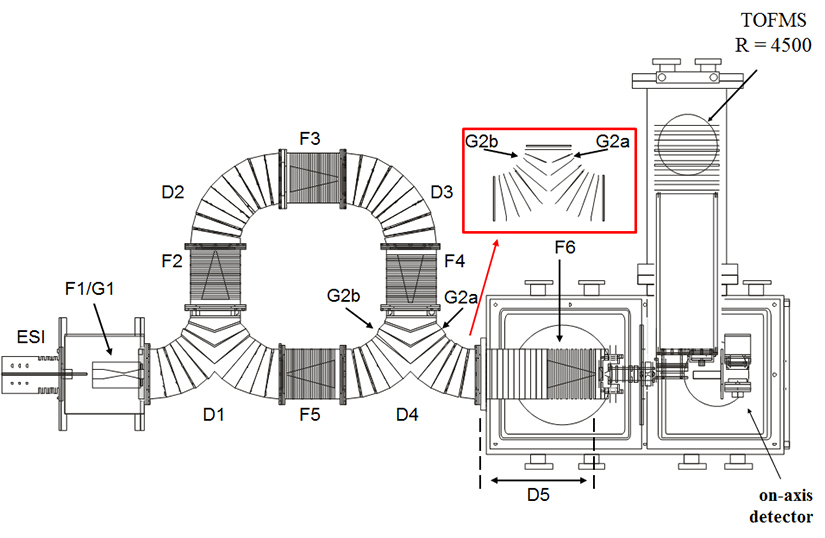
An instrument diagram is shown with ions generated by electrospray ionization (ESI) collected in a hourglass ion funnel (F1). Periodically packets of ions are pulsed into the circular drift tube containing eight distinct regions each operated at 8 V⋅cm–1. These include four curved drift regions (labeled D1–D4) and four ion funnels (labeled F2–F5). After D4 there is a short drift region operated at 9 V⋅cm–1; followed by F6 operated at 11 V⋅cm–1. Upon exiting F6, ions are then focused through a series of ion optics before being mass analyzed and detected.

There are two lenses in D4 (labeled G2a and G2b) that are isolated from the rest of the drift assembly and obtain their voltages from an external pulse generator. Ions can be transmitted around numerous cycles by switching the voltages of G2a and G2b at the appropriate time.

A home-built drift field wavedriver controls the drift field for each of the individual drift regions (D1–D4) and ion funnels (F2–F5). The field across the drift region remains constant by varying the bias of the D and F regions. Ions are propagated around the drift tube by periodically applying two separate fields to distinct sections of the drift tube. A packet of ions is introduced into the D1 region during one field application setting, and, after a specified delay, the field application setting is switched and ions can travel into the F2 region. Upon switching fields again, ions can travel into the D2 region. Ions traveling beyond or those not reaching D2 before the next field application setting are eliminated. A picture of the instrument can be found here.

With each field transition, ions at the leading and trailing edges of the transmission packet are eliminated, leaving only a narrow range of mobilities. The period of the wavedriver corresponds to the time required for ions to travel the length of one curved region and one ion funnel, which allows for the reduced mobility of the peak to be determined from the following relation, where lt and le are the lengths of the ion transmission and ion elimination regions, respectively. E is the electric field, f is the drift field application frequency (inverse of the wavedriver period), and T and P are the temperature and pressure, respectively, of the drift buffer gas.

References

Full-text formats for many of these references can be found on the Publications page. External links are provided as necessary and available.

1. Mason, E. A.; McDaniel; E. W. Transport Properties of Ions in Gases. Wiley: New York; 1988. (Link.)
2. Fenn, J. B.; Mann, M.; Meng, C. K.; Wong, S. F.; Whitehouse, C. M. Science 1988, 246, 64–71
3. Hoaglund, C. S.; Valentine, S. J.; Sporleder, C. R.; Reilly, J. P.; Clemmer, D. E. Three-Dimensional Ion Mobility/TOFMS Analysis of Electrosprayed Biomolecules, Anal. Chem. 1998, 70, 2236–2242. (Link)
4. Srebalus, C. A.; Li, J.; Marshall, W. S.; Clemmer, D. E. Gas-Phase Separations of Electrosprayed Peptide Libraries, Anal. Chem. 1999, 71, 3918–3927. (Link)
5. Hoaglund, C. S.; Valentine, S. J.; Sporleder, C. R.; Reilly, J. P.; Clemmer, D. E. Three-Dimensional Ion Mobility/TOFMS Analysis of Electrosprayed Biomolecules, Anal. Chem. 1998, 70, 2236–2242. (Link)
6. Koeniger, S. L.; Merenbloom, S. I.; Clemmer, D. E. Evidence for Many Resolvable Structures within Conformation Types of Electrosprayed Ubiquitin Ions, J. Phys. Chem B 2006, 110, 7017–7021. (Link)
7. Koeniger, S. L.; Merenbloom, S. I.; Valentine, S. J.; Jarrold, M. F.; Udseth, H.; Smith, R.; Clemmer, D. E. An IMS–IMS Analogue of MS–MS, Anal. Chem. 2006, 78, 4161–4174. (Link)
8. Koeniger, S. L.; Merenbloom, S. I.; Sevugarajan, S.; Clemmer, D. E. Transfer of Structural Elements from Compact to Extended States in Unsolvated Ubiquitin, J. Am. Chem. Soc. 2006, 128, 11713–11719. (Link)
9. Koeniger, S. L.; Clemmer, D. E. Resolution and Structural Transitions of Elongated States of Ubiquitin. J. Am. Soc. Mass Spectrom. 2007, 18, 322–331. (Link)
10. Polfer, N. C.; Bohrer, B. C.; Plasencia, M. D.; Paizs, B.; Clemmer, D. E. On the dynamics of primary structure scrambling in collision-induced dissociation of peptides. J. Phys Chem. A 2008, 112, 1286–1293. (Link)
11. Pierson, N. A.; Valentine, S. J.; Clemmer, D. E. Evidence for a Quasi-Equilibrium Distribution of States for Bradykinin [M+3H]3+ Ions in the Gas Phase. J. Phys. Chem. B, 2010, 114, 7777–7783. (Link)
12. Kim, T-Y.; Valentine, S. J.; Clemmer, D. E.; Reilly, J. P. Gas-Phase Conformation-Specific Photofragmentation of Proline-Containing Peptide Ions. J. Am. Soc. Mass Spectrom. 2010, 21, 1455–1465. (Link)
13. Bohrer, B. C.; Atlasevich, N.; Clemmer, D. E. Transitions between Elongated Conformations of Ubiquitin [M+11H]11+ Enhance Hydrogen/Deuterium Exchange. J. Phys. Chem. B 2011, 115, 4509–4515. (Link)
14. Atlasevich, N.; Holliday, A.;Valentine, S. J.; Clemmer, D. E. Collisional Activation of [14Pro+2H]2+ Clusters: Chiral Dependence of Evaporation and Fission Processes. J. Phys. Chem. B., 2012, 116, 7644–7651. (Link)
15. Merenbloom, S. I.; Koeniger, S. L.; Valentine, S. J.; Plasencia, M. D.; Clemmer, D. E. IMS–IMS and IMS–IMS–IMS/MS for Separating Peptide and Protein Fragment Ions, Anal. Chem. 2006, 78, 2802–2809. (Link)
16. Merenbloom, S. I.; Bohrer, B. C.; Koeniger, S. L.; Clemmer, D. E. Assessing the Peak Capacity of IMS–IMS Separations of Tryptic Peptide Ions in 300 K He, Anal. Chem. 2007, 79, 515–522. (Link)
17. Merenbloom, S. I.; Koeniger, S. L.; Bohrer, B. C.; Valentine, S. J.; Clemmer, D. E. Improving the Efficiency of IMS–IMS by a Combing Technique. Anal. Chem. 2008, 80, 1918–1927. (Link)
18. Kurulugama, R. T.; Valentine, S. J.; Sowell, R. A.; Clemmer, D. E. Development of a high-throughput IMS–IMS–MS approach for analyzing mixtures of biomolecules. J. Proteomics, 2008, 71, 318–331. (Link)
19. Valentine, S. J.; Kurulugama, R. T.; Bohrer, B. C.; Merenbloom, S. I.; Sowell, R. A.; Mechref, Y; Clemmer, D. E. Developing IMS–IMS–MS for rapid characterization of abundant proteins in human plasma. Int. J. Mass Spectrom. 2009, 283, 149–160. (Link)
20. Trimpin, S.; Tan, B.; Bohrer, B. C.; O�Dell, D. K.; Merenbloom, S. I.; Pazos, M. X.; Clemmer, D. E.; Walker, J.M. Profiling of Phospholipids and Related Lipid Structures using Multidimensional Ion Mobility Spectrometry–Mass Spectrometry. Int. J. Mass Spectrom. 2009, 287, 58–69. (Link)
21. Li, Z.; Valentine, S. J.; Clemmer, D. E. Complexation of Amino Compounds by 18C6 Improves Selectivity by IMS–IMS–MS: Application to Petroleum Characterization. J. Am. Soc. Mass. Spectrom. 2011, 22, 817–27. (Link)
22. Bohrer, B. C.; Clemmer, D. E. Shift Reagents for Multidimensional Ion Mobility Spectrometry–Mass Spectrometry Analysis of Complex Peptide Mixtures: Evaluation of 18-Crown-6 Ether Complexes. Anal. Chem., 2011, 83, 5377–5385. (Link)
23. Merenbloom, S. I.; Glaskin, R. S.; Henson, Z. B.; Clemmer, D. E. High-Resolution Ion Cyclotron Mobility Spectrometry. Anal. Chem. 2009, 81, 1482–1487. (Link)
24. Glaskin, R. S.; Valentine, S. J.; Clemmer, D. E. A Scanning Frequency Mode for Ion Cyclotron Mobility Spectrometry. Anal. Chem. 2010, 82, 8266–8271. (Link)
25. Zucker, S. M.; Lee, S.; Webber, N.; Valentine, S. J.; Reilly, J. P. Clemmer, D. E. An Ion Mobility/Ion Trap/Photodissociation Instrument for Characterization of Ion Structure. J. Am. Soc. Mass Spectrom., 2011, 22, 1477–1485. (Link)
26. Lee, S.; Valentine, S. J.; Zucker, S. M.; Webber, N.; Reilly, J. P.; Clemmer, D. E. Extracted Fragment Ion Mobility Distributions: A New Method for Complex Mixture Analysis. Int. J. Mass Spectrom. 2012, 309, 154–160. (Link)
27. Lee, S.; Valentine, S. J.; Reilly, J. P.; Clemmer, D. E. Analyzing a Mixture of Disaccharides by IMS–VUVPD–MS. Int. J. Mass Spectrom. 2012, 309, 161–167. (Link)